import os
os.environ["KERAS_BACKEND"] = "tensorflow"
import tensorflow as tf
import keras
import numpy as np
import matplotlib.pyplot as plt
from sklearn.datasets import make_swiss_roll
from math import piFlow matching with conditioning
In the previous exercises, we trained a normalizing flow and a flow matching models to reproduce one distribution.
In this example, we will expand the concept a little bit and show that a single generative model can be trained to generate different distributions, by conditioning on additional variables.
The data
We will use the swiss roll data distribution available from the sklearn library. This distribution generates samples in 3D, but we will only focus on a 2D projection, since the third dimension is not very interesting.
n_samples=1_000data, _ = make_swiss_roll(n_samples, noise=1)
data = data[:,[0, -1]]
fig=plt.scatter(data[:,0], data[:,1])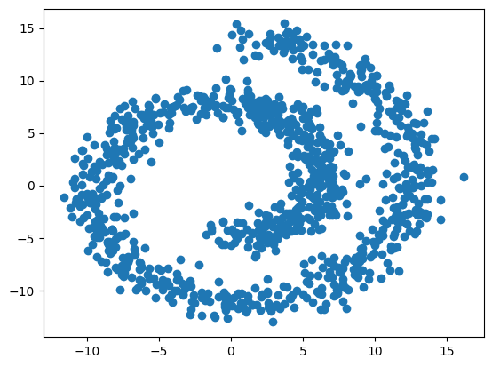
To show that generative models like flow matching can use other base distributions than the normal, we will also create a custom base distribution that samples values along a circle (a ring).
def make_ring(n_samples):
    u = np.random.uniform(low=0, high=2*pi, size=(n_samples,1))
    r = np.random.uniform(low=9, high=10, size=(n_samples,1))
    x = r * np.sin(u)
    y = r * np.cos(u)
    return np.concatenate([x, y], axis=-1)


base = make_ring(n_samples)
fig=plt.scatter(base[:,0], base[:,1])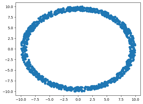
The model
The model is the same as in the datasaurus flow matching exercise except that the velocity network also accepts additional variables that we here call condition. This allows us to train the network to generate different distributions, depending on the values of condition that we choose.
class FlowMatching(keras.Model):
    def __init__(self, n_units, n_layers, dim=2):
        """ Initiate the flow matching model object

        Parameters
        ----------
        n_units: int
            Number of units per each layer of the velocity MLP
        n_layers: int
            Number of layers of the velocity MLP
        dim: int
            Number of output dimensions (by default 2 because the datasaurus lives in 2D)
        """
        super(FlowMatching, self).__init__()
        self.dim = dim
        self.velocity = keras.Sequential(
            [keras.layers.Dense(n_units, activation="elu") for _ in range(n_layers)]
            )
        self.velocity.add(keras.layers.Dense(dim))

    def call(self, inputs):
        """ Call the velocity vector

        Parameters
        ----------
        inputs: dict
            x_0: samples from the base distribution
            x_1: samples from the data distribution
            t:   samples of the time variable between [0, 1]
            condition: some conditioning variables


        Returns the velocity vector
        """
        x_0, x_1, t, condition = inputs.values()
        x_t = (1-t)*x_0 + t*x_1
        x = keras.ops.concatenate([x_t, t, condition], axis=-1)
        return self.velocity(x)

    def step(self, x, t, dt, condition):
        """ Make one step using the midpoint ODE solver

        Parameters
        ----------
        x: tensor/array (batch_size, dim)
            Samples of the variable x_t
        t: tuple/array (batch_size,)
            Samples of the time variable between [0, 1]
        dt: float
            The size of the time step
        condition: some conditioning variables

        Returns: tensor/array (batch_size, dim)
            Samples of the variable x_{t+dt}
        """

        t_start = np.zeros_like(x) + t
        input_start = keras.ops.concatenate([x, t_start, condition], axis=-1)
        v = self.velocity(input_start)
        x_mid = x + v * dt / 2

        t_mid = t_start + dt / 2
        input_mid = keras.ops.concatenate([x_mid, t_mid, condition], axis=-1)
        v = self.velocity(input_mid)
        x_end = x + v * dt

        return x_end

    def run(self, x, steps, condition):
        """ Run the ODE solver from t=0 to t=1

        Parameters
        ----------
        x: tensor/array (batch_size, dim)
            Samples from the base distribution, x_0
        steps: int
            Number of steps to make between t=0 and t=1
        condition: some conditioning variables

        Returns: tensor/array (batch_size, dim)
            Samples x_1 ~ p_1
        """

        time = np.linspace(0, 1, steps+1)
        output = []
        output.append(x)
        for i in range(steps):
            x = self.step(x, time[i], time[i+1]-time[i], condition)
            output.append(x)

        return output

    def sample(self, n_samples, steps, condition):
        """ Sample from the learned distribution

        Parameters
        ----------
        n_samples: int
            Number of samples to take
        steps: int
            Number of steps to make between t=0 and t=1 in the ODE
        condition: some conditioning variables

        Returns (array (batch_size, steps+1, dim)
            Samples of x_t ~ p_t
        """
        condition = np.array(condition)[np.newaxis,...]
        condition = np.repeat(condition, repeats=n_samples, axis=0)

        x_0 = make_ring(n_samples)
        x_1 = self.run(x_0, steps, condition)
        return np.array(x_1).swapaxes(0, 1)
Once we defined our model class, we can instantiate a new flow matching model object.
flow = FlowMatching(n_units=64, n_layers=8)Training
Similarly as in the datasaurus exercise, we will use a dataset object to do our sampling. Here, we will always generate a fresh batch of new data - from the swiss roll distribution, and from the ring distribution.
We will also make a twist: We will randomly sample values of 1 or -1 for the x and y coordinate, which we use to scale the swiss roll data. This will produce 4 different variations of the swiss roll data, reflected along and \(x\) or \(y\) axis. The values of this scale will be passed to the velocity network as condition.
Otherwise, the rest is the same as with the datasaurus.
class DataSet(keras.utils.PyDataset):
    def __init__(self, batch_size, n_batches):
        super().__init__()
        self.n_batches=n_batches
        self.batch_size = batch_size

    @property
    def num_batches(self):
        return self.n_batches

    def __getitem__(self, index):
        data, _ = make_swiss_roll(self.batch_size, noise=1)
        data=data[:,[0, -1]]

        condition=np.random.choice([1, -1], size=(batch_size, 2))
        data=condition * data

        base=make_ring(data.shape[0])

        t=np.random.uniform(low=0, high=1, size=data.shape[0])
        t=np.repeat(t[:,np.newaxis], repeats=data.shape[1], axis=1)

        target = data - base
        return dict(x_0=base, x_1=data, t=t, condition=condition), target
Next, we instantiate the dataset object, and define our schedule and optimizer, and compile the model.
epochs=20
batches=1000
batch_size=512

dataset=DataSet(batch_size=batch_size, n_batches=epochs*batches)

schedule = keras.optimizers.schedules.CosineDecay(initial_learning_rate=0.01, decay_steps=epochs*batches)
optimizer = keras.optimizers.Adam(schedule, global_clipnorm=1.0)

flow.compile(
    optimizer=optimizer,
    loss=keras.losses.MeanSquaredError()
)
Again, the same as with the datasaurus exercise, we can call the .fit method to train the model.
history=flow.fit(x=dataset, epochs=epochs, steps_per_epoch=batches)Epoch 1/20 1000/1000 ━━━━━━━━━━━━━━━━━━━━ 5s 4ms/step - loss: 67.5142 Epoch 2/20 1000/1000 ━━━━━━━━━━━━━━━━━━━━ 4s 4ms/step - loss: 60.5823 Epoch 3/20 1000/1000 ━━━━━━━━━━━━━━━━━━━━ 4s 4ms/step - loss: 59.2506 Epoch 4/20 1000/1000 ━━━━━━━━━━━━━━━━━━━━ 4s 4ms/step - loss: 58.8516 Epoch 5/20 1000/1000 ━━━━━━━━━━━━━━━━━━━━ 4s 4ms/step - loss: 58.4735 Epoch 6/20 1000/1000 ━━━━━━━━━━━━━━━━━━━━ 4s 4ms/step - loss: 58.0877 Epoch 7/20 1000/1000 ━━━━━━━━━━━━━━━━━━━━ 4s 4ms/step - loss: 57.6959 Epoch 8/20 1000/1000 ━━━━━━━━━━━━━━━━━━━━ 3s 3ms/step - loss: 57.6651 Epoch 9/20 1000/1000 ━━━━━━━━━━━━━━━━━━━━ 4s 4ms/step - loss: 57.3689 Epoch 10/20 1000/1000 ━━━━━━━━━━━━━━━━━━━━ 4s 4ms/step - loss: 57.1357 Epoch 11/20 1000/1000 ━━━━━━━━━━━━━━━━━━━━ 4s 4ms/step - loss: 56.9357 Epoch 12/20 1000/1000 ━━━━━━━━━━━━━━━━━━━━ 4s 4ms/step - loss: 56.5468 Epoch 13/20 1000/1000 ━━━━━━━━━━━━━━━━━━━━ 4s 4ms/step - loss: 56.4292 Epoch 14/20 1000/1000 ━━━━━━━━━━━━━━━━━━━━ 3s 3ms/step - loss: 56.2061 Epoch 15/20 1000/1000 ━━━━━━━━━━━━━━━━━━━━ 4s 4ms/step - loss: 56.1961 Epoch 16/20 1000/1000 ━━━━━━━━━━━━━━━━━━━━ 4s 4ms/step - loss: 56.1195 Epoch 17/20 1000/1000 ━━━━━━━━━━━━━━━━━━━━ 4s 4ms/step - loss: 56.1653 Epoch 18/20 1000/1000 ━━━━━━━━━━━━━━━━━━━━ 4s 4ms/step - loss: 55.8236 Epoch 19/20 1000/1000 ━━━━━━━━━━━━━━━━━━━━ 4s 4ms/step - loss: 55.8725 Epoch 20/20 1000/1000 ━━━━━━━━━━━━━━━━━━━━ 4s 4ms/step - loss: 55.6168
f=plt.plot(history.history["loss"])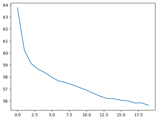
Now that we fitted the model, let’s see the samples it generates!
Here we will loop over the possible combinations of the condition which is either -1 or 1 for \(x\) and \(y\) coordinate - leading to 4 different distributions produced by the flow matching model.
fig, axs = plt.subplots(2, 2, sharex=True, sharey=True)
for i, x_scale in enumerate([1, -1]):
    for j, y_scale in enumerate([1, -1]):
        condition = [x_scale, y_scale]
        x = flow.sample(n_samples=n_samples, steps=100, condition=condition)
        axs[i,j].scatter(x[:, -1, 0], x[:, -1, 1], s=10, alpha=0.5)
        axs[i,j].set_title("x scale: {}, y scale {}".format(x_scale, y_scale))
fig.tight_layout()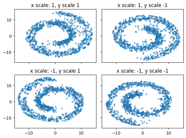
Further exercises
- Here we only scaled the data by 2 values (-1 or 1) in two directions (\(x\) and \(y\)). However, there is nothing that can stop us from using different values. Try to replace the line
condition=np.random.choice([1, -1], size=(batch_size, 2))with some other transformation (for example, generate values from a uniform distribution between -1 and 1). What do you think the network will learn? Try it for yourself. - The swiss roll distribution generates 3D data. In this exercise, we only used 2 of the axes and neglected the third one. Try to change to model so that you can actually reproduce the swiss role in 3D (note: you will also need to change the base distribution to be 3D).