Generative Neural Networks

Šimon Kucharský

Generative models

Learn \(p_X\) given a set of training data \(x_i, \dots, x_n\)

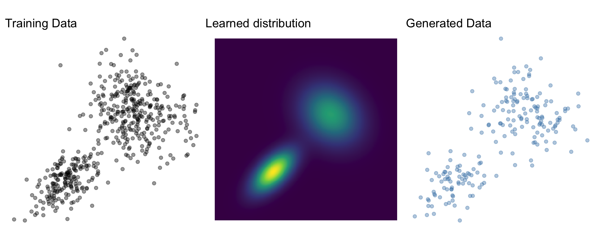
• Sampling \(x \sim p_X\)
• Density evaluation \(p_X(x)\)

Mixture model

Weighted sum of multiple simpler distributions, e.g., Normal \[p_X(X) = \sum_k^K w_k \times \text{Normal}(X; \mu_k, \sigma_k)\]

• Sampling and evaluating straightforward
• Theoretically can represent any distribution
• Practically, does not scale well

Many architectures

• Markov random fields (Li, 2009)
• Generative adversarial networks (GAN, Goodfellow et al., 2014)
• Variational autoencoders (VAE, Kingma et al., 2013)
• Diffusion models (Song et al., 2020)
• Consistency models (Song et al., 2023)
• Normalizing flows (Kobyzev et al., 2020; Papamakarios et al., 2021)
• Flow matching (Lipman et al., 2022)

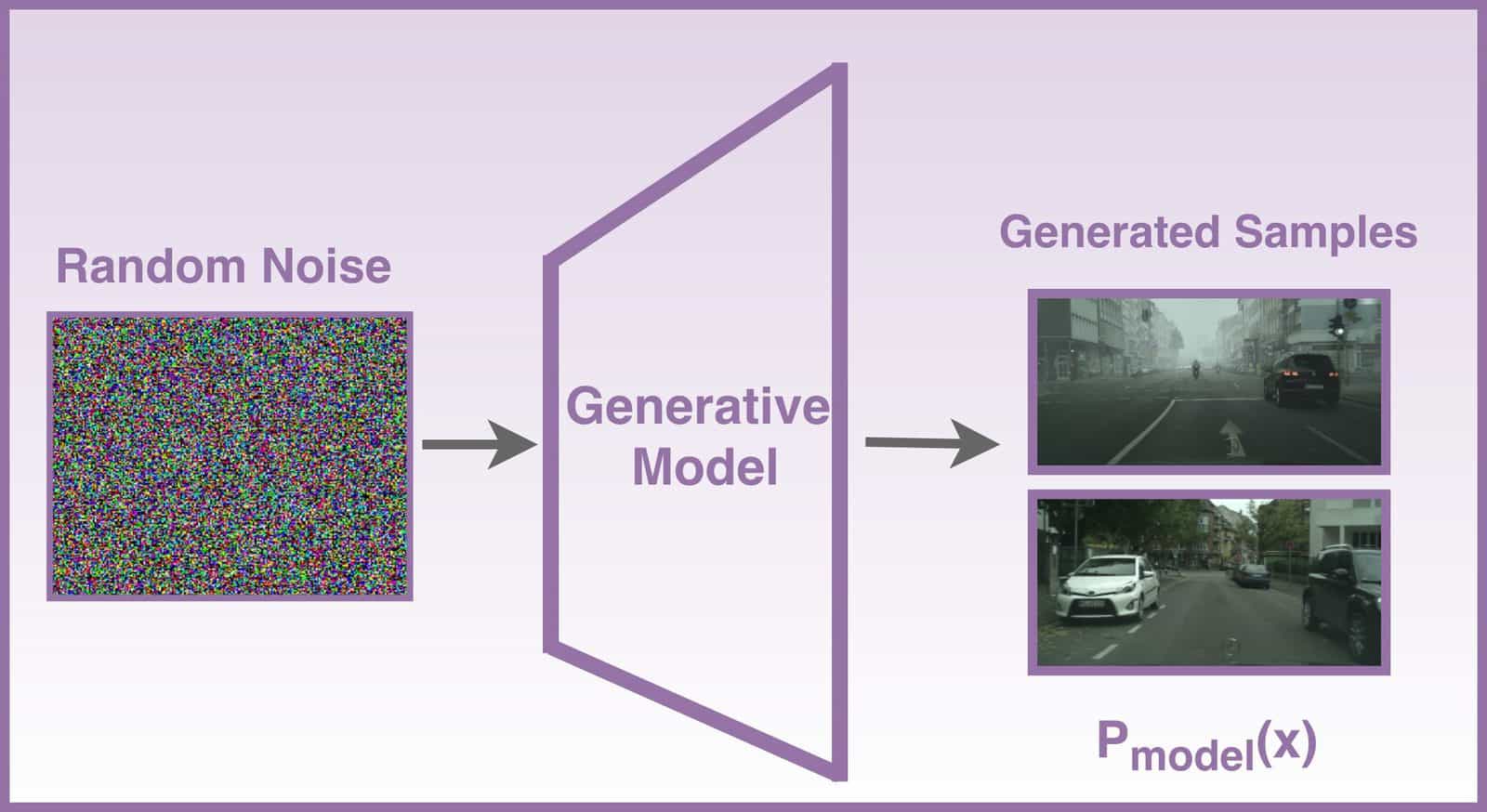
Common idea

Map \(p_X\) to a base distribution \(p_Z\) through some operation \(g\)

\[ x \sim g(z) \text{ where } z \sim p_Z \]

Source: learnopencv.com

Normalizing flows

Normalizing flows

Built on invertible transformations of random variables

• Find \(f\) such that \(f(X) = Z \sim \text{Normal}(0, I)\)
  • \(f\) normalizes \(X\)

 

\(f\)

 

\[\rightarrow\]

Figure 1: Forward direction

Sampling

• Sample \(z \sim p_Z\) (e.g., Normal)
• Obtain \(x = f^{-1}(z)\)

 

\(f^{-1}\)

 

\[\leftarrow\]

Figure 2: Backward direction

Density evaluation

Change of variables formula

\[ p_X(x) = p_Z(f(x)) \left| \det{J}_f(x) \right| \]

• Express \(p_X\) using \(p_Z\) and the transform \(f\)
• \(\left| \det{J}_f(x) \right|\): Absolute value of the determinant of the Jacobian matrix
  • “Jacobian” for short
  • Volume correction term

Change of variables - intuition

\[Z \sim \text{Uniform}(0, 1)\]

Change of variables - intuition

\[Z \sim \text{Uniform}(0, 1)\]

Change of variables - intuition

\[Z \sim \text{Uniform}(0, 1)\]

\[X = 2Z - 1\]

Change of variables - intuition

\[Z \sim \text{Uniform}(0, 1)\]

\[X = 2Z - 1\]

Change of variables - affine transform

\[f: Z = a X + b\]

• shift by \(b\): no effect
• scale by a constant \(a\): multiply by \(a\)

\[p_X(x) = p_Z(f(x)) \times a\]

Change of variables - affine transform

Example

\[ \scriptsize \begin{aligned} p_Z(z) & = \frac{1}{\sqrt{2\pi}} \exp\left(-\frac{1}{2} z^2 \right) \\[10pt] f: Z & = \frac{(X - \mu)}{\sigma} \\ \end{aligned} \]

\[ \scriptsize \begin{aligned} p_X(x) & = p_Z(f(x)) \times a \\[10pt] & = \frac{1}{\sqrt{2\pi}} \exp\left(-\frac{1}{2} f(x)^2 \right) \times a \\[10pt] & = \frac{1}{\sigma\sqrt{2\pi}} \exp\left(-\frac{1}{2} \left(\frac{x-\mu}{\sigma}\right)^2 \right) \end{aligned} \]

Change of variables - more formally

\[ p_X(x) = p_Z(f(x)) \left| \frac{d}{dx} f(x) \right| \]

Change of variables - more formally

\[ p_X(x) = p_Z(f(x)) \left| \frac{d}{dx} f(x) \right| \]

Example

\[ \scriptsize \begin{align} f: Z & = \log(X) \\[10pt] p_Z(z) & = \frac{1}{\sqrt{2\pi}} \exp\left(-\frac{1}{2} z^2 \right) \end{align} \]

\[ \scriptsize \begin{align} \frac{d}{dx} f(x) & = \frac{d}{dx} \log(x) = \frac{1}{x} \\[10pt] p_X(x) & = \frac{1}{x\sqrt{2\pi}} \exp\left(-\frac{1}{2} \log(x)^2\right) \end{align} \]

Change of variables - multivariate

\[ p_X(x) = p_Z(f(x)) \left| \det{J}_f(x) \right| \]

\[ J_f(x) = \begin{bmatrix} \frac{\partial z_1}{\partial x_1} & \dots & \frac{\partial z_1}{\partial x_K} \\ \vdots & \ddots & \vdots \\ \frac{\partial z_K}{\partial x_1} & \dots & \frac{\partial z_K}{\partial x_K} \end{bmatrix} \]

Change of variables - multivariate

\[f\left(\begin{bmatrix}x_1 \\ x_2\end{bmatrix}\right) = \begin{bmatrix} x_1^2 x_2 \\ 3x_1 + \sin x_2 \end{bmatrix} = \begin{bmatrix}z_1 \\ z_2\end{bmatrix}\]

\[J_f(x) = \begin{bmatrix} \frac{\partial z_1}{\partial x_1} & \frac{\partial z_1}{\partial x_2} \\ \frac{\partial z_2}{\partial x_1} & \frac{\partial z_2}{\partial x_2} \end{bmatrix} = \begin{bmatrix} 2x_1x_2 & x_1^2 \\ 3 & \cos x_2 \end{bmatrix} \]

Normalizing flow

\[ p_X(x) = p_Z(f(x)) \left| \det{J}_f(x) \right| \]

Define a \(f\) as a neural network with trainable weights \(\phi\)

Training

Maximum likelihood (or rather: negative log likelihood)

\[ \arg \min_\phi - \sum_{i=1}^n \log p_Z(f(x_i \mid \phi)) + \log \left| \det{J}_f(x_i \mid \phi) \right| \]

Flow \(f\)

Challenge

• Sampling: Invertible (\(f^{-1}\))
• Training:
  • Differentiable
  • Computationally efficient jacobian
• Expressive to represent non-trivial distributions

Flow composition

Invertible and differentiable functions are “closed” under composition

\[ f = f_L \circ f_{L-1} \circ \dots \circ f_1 \\ \]

 

\(f_1\)

 

\(f_2\)

 

\(f_3\)

 

\(\rightarrow\)

\(\rightarrow\)

\(\rightarrow\)

Figure 3: Flow composition in forward direction

Flow composition - inverse

To invert a flow composition, we invert individual flows and run them in the opposite order

\[ f^{-1} = f_1^{-1} \circ f_2 ^{-1} \circ \dots \circ f_L^{-1} \\ \]

 

\(f_1^{-1}\)

 

\(f_2^{-1}\)

 

\(f_3^{-1}\)

 

\(\leftarrow\)

\(\leftarrow\)

\(\leftarrow\)

Figure 4: Flow composition in backward (inverse) direction

Flow composition - Jacobian

• Chain rule \[ \left| \det{J}_f(x) \right| = \left| \det \prod_{l=1}^L J_{f_l}(x)\right| = \prod_{l=1}^L \left| \det{J}_{f_l}(x)\right| \]

• if we have a Jacobian for each individual transformation, then we have a Jacobian for their composition \[ \arg \min_\phi \sum_{i=1}^n \log p_Z(f(x_i \mid \phi)) + \sum_{l=1}^L \log \left| \det{J}_{f_l}(x_i \mid \phi) \right| \]

Linear flow

\[ f(x) = Ax + b \]

• inverse: \(f^{-1}(z) = A^{-1}(x - b)\)

• Jacobian: \(\left| \det{J}_f(x) \right| = \left| \det{A} \right|\)

• Limitations:

  1. Not expressive (composition of linear functions is a linear function)
  2. Jacobian/inverse may be in \(\mathcal{O}(p^3)\)

Coupling flows

• Increasing expresiveness while potentially decreasing computational costs
• A coupling flow is a way to construct non-linear flows

1. Split the data in two disjoint subsets: \(x = (x_A, x_B)\)
2. Compute parameters conditionally on one subset: \(\theta(x_A)\)
3. Apply transformation to the other subset: \(z_B = f(x_B \mid \theta(x_A))\)
4. Concatenate \(z = (x_A, z_B)\)

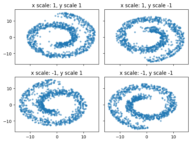
Coupling flow: Forward

Coupling flow: Inverse

Coupling flow trick

• Jacobian

\[ J_f = \begin{bmatrix} \text{I} & 0 \\ \frac{\partial}{\partial x_A}f(x_B \mid \theta(x_A)) & J_f(x_B \mid \theta(x_A)) \end{bmatrix} \]

• Determinant

\[ \det{J}_f = \det(\text{I}) \times \det{J}_f(x_B \mid \theta(x_A)) = \det{J}_f(x_B \mid \theta(x_A)) \]

Coupling flow trick

• \(f(x_B\mid\theta(x_A))\) needs to be differentiable and invertible
  • easy to calculate determinant Jacobian…
• \(\theta(x_A)\) can be arbitrarily complex
  • non-linear,
  • non-invertible
  • \(\rightarrow\) neural network

• Stack multiple coupling blocks and permute \(x_{A}\) and \(x_{B}\)

Affine coupling (Dinh et al., 2016)

• \(\theta(x_A)\): Trainable coupling networks, e.g., MLP

  • Output: Shift \(\mu\) and scale \(\sigma\)

• Linear (affine) transform function \(f(x_B\mid\theta(x_A)) = \frac{x_B - \mu(x_A)}{\sigma(x_A)}\)

• Jacobian: \(-\log{\sigma(x_A)}\)

Spline coupling (Müller et al., 2019)

• Transformation: Splines
  • “Piecewise polynomials”
• More expressive
• Easier to overfit
• Slower at training and inference

Figure from Durkan et al. (2019)

Exercise - Moons

Build your own affine coupling normalizing flow!

Forward

Backward

Idea

• Normalizing flows transform X into Z in a set of discrete steps
• But why not take one smooth/continuous transformation?

Flow matching (Lipman et al., 2022)

Essentials from an extensive tutorial by Lipman et al. (2024) available at https://neurips.cc/virtual/2024/tutorial/99531.

Flow matching

• Defines a flow that transforms a distribution over time
  • \(p_{t=0} = p_z\) - Base distribution
  • \(p_{t=1} = q = p_x\) - Data distribution

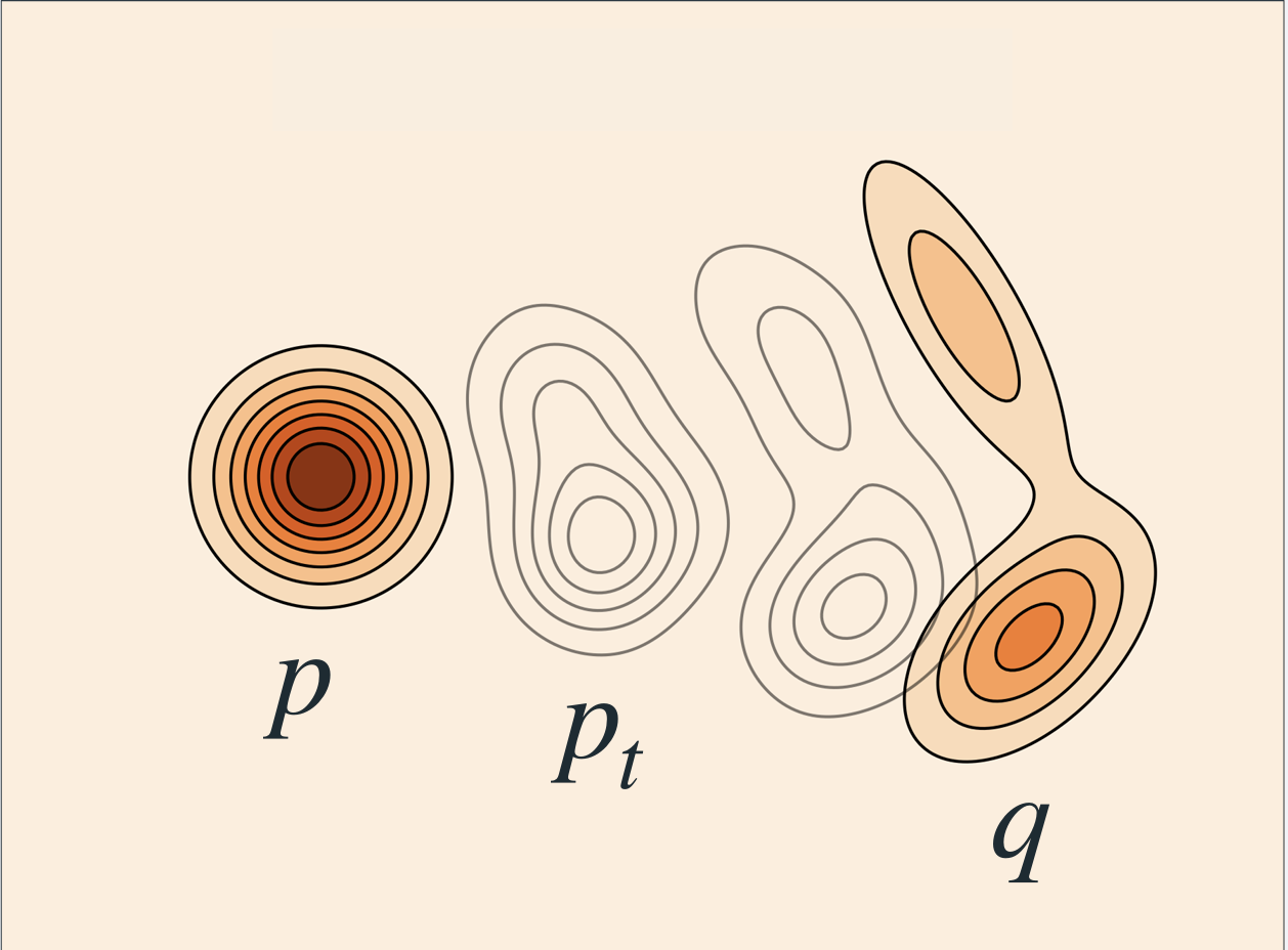
Lipman et al. (2024)

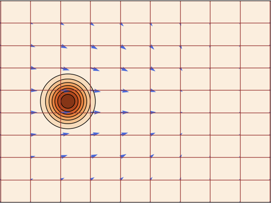
Flow and velocity

• Flow defines \(X_t = \phi_t(X_0)\)
• Time dependent vector field: \(\frac{d}{dt} \phi_t(x) = u_t(\phi_t(x))\)
• Model \(u_t\) with a neural network

Lipman et al. (2024)

Flow matching

\[ \begin{aligned} \mathbb{E}_{t, X_t}|| u_{t,\theta}(X_t) - u_t(X_t) ||^2 \\ t\sim\text{Uniform}(0,1) \\ X_t \sim p_t(X_t) \end{aligned} \]

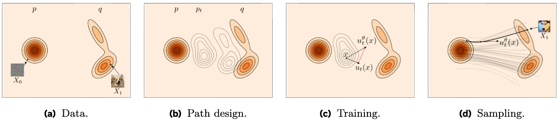
Lipman et al. (2024)

Conditional Flow Matching

Linear probability path

\[X_t = (1-t) X_0 + t X_1\]

Velocity

\[u_t(X_t \mid X_1, X_0) = X_1 - X_0\]

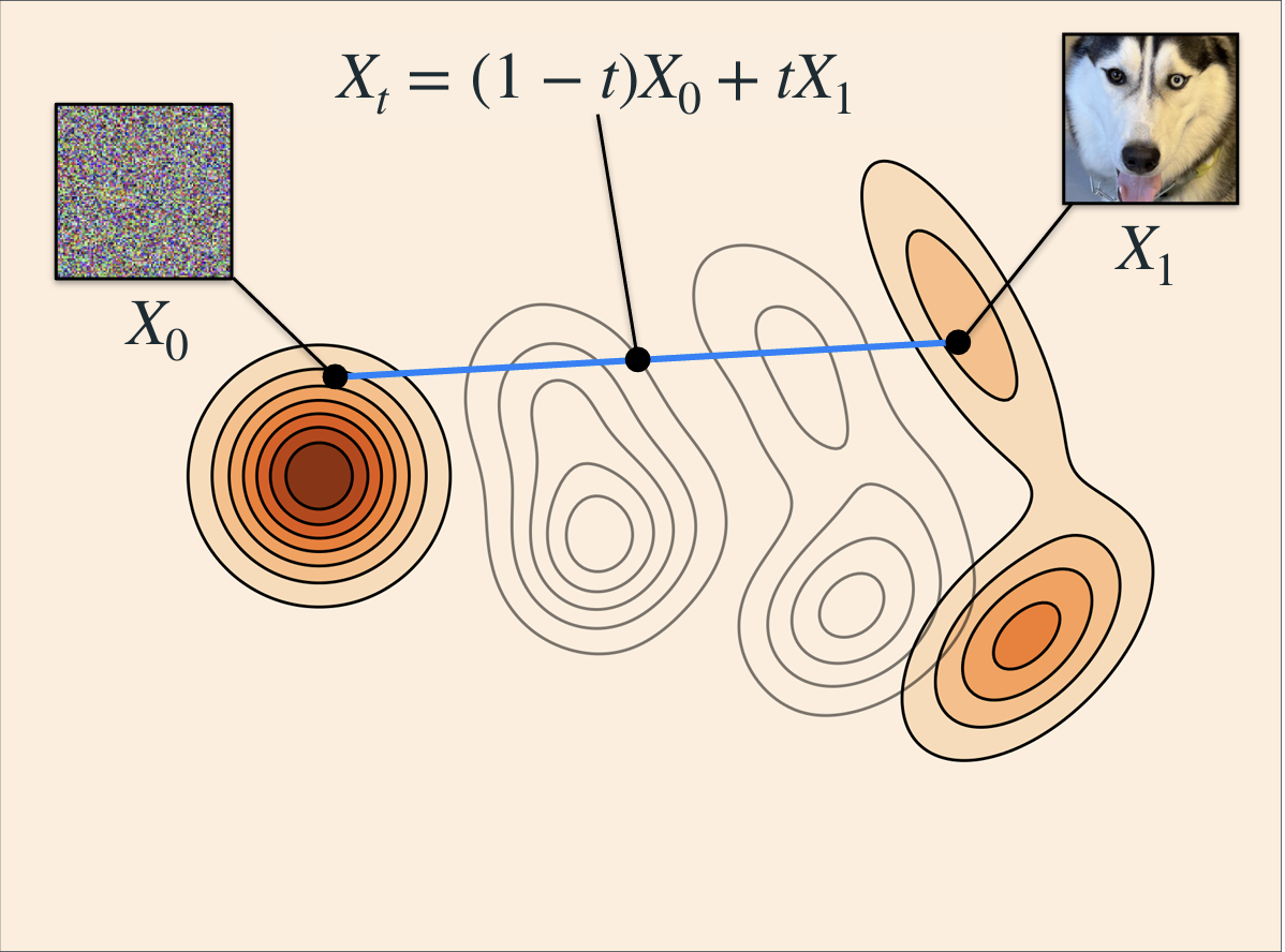
Lipman et al. (2024)

Conditional Flow Matching

\[ \begin{aligned} \mathbb{E}_{t, X_t}|| u_{t,\theta}\big(\underbrace{(1-t) X_0 + t X_1)}_{X_t}\big) - (\underbrace{X_1-X_0}_{u_t}) ||^2 \\ t\sim\text{Uniform}(0,1) \\ X_0 \sim p_0 \\ X_1 \sim p_1 \end{aligned} \]

Conditional vs Marginal paths

Conditional path

Marginal path

Figure 5: Fjelde et al. (2024)

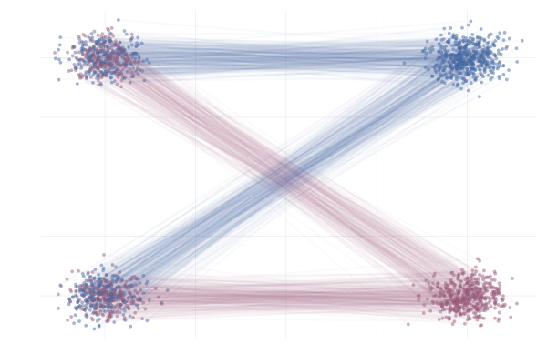
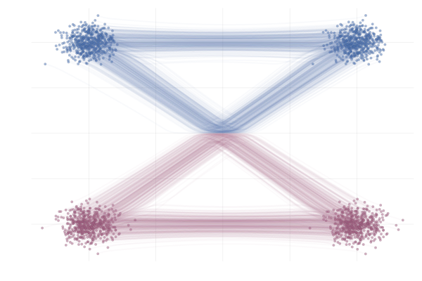
Optimal transport

• Independent coupling \(p(X_0, X_1) = p(X_0) p(X_1)\)
• Optimal transport coupling \(p(X_0, X_1) = \pi(X_0, X_1)\)
  • Minimise transport cost (e.g., Wasserstein distance)
  • For batches (Pooladian et al., 2023)

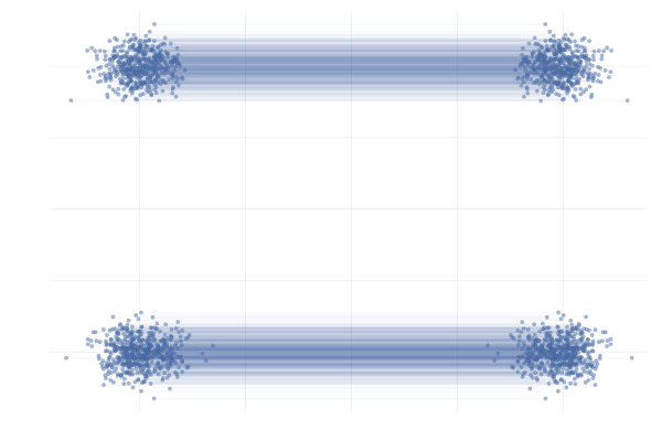
Figure 6: Fjelde et al. (2024)

Exercise

Exercise

References

Dinh, L., Sohl-Dickstein, J., & Bengio, S. (2016). Density estimation using real nvp. arXiv Preprint arXiv:1605.08803.

Durkan, C., Bekasov, A., Murray, I., & Papamakarios, G. (2019). Neural spline flows. Advances in Neural Information Processing Systems, 32.

Fjelde, T., Mathieu, E., & Dutordoir, V. (2024). An Introduction to Flow Matching. https://mlg.eng.cam.ac.uk/blog/2024/01/20/flow-matching.html

Goodfellow, I. J., Pouget-Abadie, J., Mirza, M., Xu, B., Warde-Farley, D., Ozair, S., Courville, A., & Bengio, Y. (2014). Generative adversarial nets. Advances in Neural Information Processing Systems, 27.

Kingma, D. P., Welling, M., et al. (2013). Auto-encoding variational bayes. Banff, Canada.

Kobyzev, I., Prince, S. J., & Brubaker, M. A. (2020). Normalizing flows: An introduction and review of current methods. IEEE Transactions on Pattern Analysis and Machine Intelligence, 43(11), 3964–3979.

Li, S. Z. (2009). Markov random field modeling in image analysis. Springer Science & Business Media.

Lipman, Y., Chen, R. T., Ben-Hamu, H., Nickel, M., & Le, M. (2022). Flow matching for generative modeling. arXiv Preprint arXiv:2210.02747.

Lipman, Y., Havasi, M., Holderrieth, P., Shaul, N., Le, M., Karrer, B., Chen, R. T. Q., Lopez-Paz, D., Ben-Hamu, H., & Gat, I. (2024). Flow matching guide and code. https://arxiv.org/abs/2412.06264

Müller, T., McWilliams, B., Rousselle, F., Gross, M., & Novák, J. (2019). Neural importance sampling. ACM Transactions on Graphics (ToG), 38(5), 1–19.

Papamakarios, G., Nalisnick, E., Rezende, D. J., Mohamed, S., & Lakshminarayanan, B. (2021). Normalizing flows for probabilistic modeling and inference. Journal of Machine Learning Research, 22(57), 1–64.

Pooladian, A.-A., Ben-Hamu, H., Domingo-Enrich, C., Amos, B., Lipman, Y., & Chen, R. T. (2023). Multisample flow matching: Straightening flows with minibatch couplings. arXiv Preprint arXiv:2304.14772.

Song, Y., Dhariwal, P., Chen, M., & Sutskever, I. (2023). Consistency models.

Song, Y., Sohl-Dickstein, J., Kingma, D. P., Kumar, A., Ermon, S., & Poole, B. (2020). Score-based generative modeling through stochastic differential equations. arXiv Preprint arXiv:2011.13456.