Deep Learning

Introduction

Šimon Kucharský

Shahab et al. (2024)

Deep Learning in Python

Python frameworks

• PyTorch
• TensorFlow
• JAX
• keras

PyTorch

• created by Meta (formerly Facebook)
• easy to learn
• focus on research prototypes
• models are not compiled

TensorFlow

• created by Google
• easy to learn
• focus on production
• models are compiled

JAX

• created by Google
• pure, functional approach
• JIT compiled
• fastest in runtime
• most difficult to learn

keras

• created by Google
• API library
• Uses PyTorch, TensorFlow, or jax as a backend

Python

import os
os.environ["KERAS_BACKEND"] = "tensorflow" # torch, jax
import keras

keras

• created by Google
• API library
• Uses PyTorch, TensorFlow, or jax as a backend

Terminal

conda env config vars set KERAS_BACKEND=jax

Python

import keras

Tensors

• All of Deep Learning revolves around “Tensors”
• Similar to arrays in numpy
• Additional features:
  • Values and gradients
  • Can be stored on GPUs (optional)

Tensors

Python

import os
os.environ["KERAS_BACKEND"] = "tensorflow"
import keras

x = keras.ops.zeros((16, 2))
x.shape # TensorShape([16, 2])
x.device # device:CPU:0

• First axis almost always batch_size (think “sample size”)
• Other axes contextual (timepoint, feature, variable, row, column, etc)

Neural networks

The anatomy of neural networks

Neuron

Regression + non-linear activation

Perceptron

Multiple regressions + non-linear activations

\[ \begin{aligned} z_k &= \sigma \Big(b_k + \sum_{j=1}^J W_{jk}x_j\Big)\\ z &= \sigma \Big(b + x W'\Big) \end{aligned} \]

Perceptron in code

Python

import keras

network = keras.models.Sequential([
    keras.Input((3,)),
    keras.layers.Dense(5, activation="relu"),
])
network.summary()

x = keras.random.normal((100, 3))
x.shape # TensorShape([100, 3])

z = network(x)
z.shape # TensorShape([100, 5])

Multi-Layer Perceptron

Multiple “layers” of perceptrons

Multi-Layer Perceptron

Function composition

\[ \begin{aligned} z & = f(x) \text{ where } f = f_L \circ f_{L-1} \circ \dots \circ f_1 \\ z & = f_L(\dots(f_2(f_1(x)))) \\ \end{aligned} \]

• \(W_{jk}^l\): weight of the input \(j\) to the output \(k\) in the layer \(l\)

Multi-Layer Perceptron in Code

Python

import keras

network = keras.models.Sequential([
    keras.Input((3,)),
    keras.layers.Dense(4, activation="relu"),   # 3 inputs, 4 outputs
    keras.layers.Dense(4, activation="relu"),   # 4 inputs, 4 outputs
    keras.layers.Dense(2, activation="softmax") # 4 inputs, 2 outputs
])
network.summary()

x = keras.random.normal((100, 3))
x.shape # TensorShape([100, 3])

z = network(x)
z.shape # TensorShape([100, 2])

Multi-Layer Perceptron in Code

Python

import keras

network = keras.models.Sequential([
    keras.Input((3,)),
    keras.layers.Dense(4, activation="relu"),   # 3 inputs, 4 outputs
    keras.layers.Dense(4, activation="relu"),   # 4 inputs, 4 outputs
    keras.layers.Dense(2, activation="softmax") # 4 inputs, 2 outputs
])
network.summary()

x = keras.random.normal((100, 3))
x.shape # TensorShape([100, 3])

z = network(x) 
z.shape # TensorShape([100, 2])

Activation functions

Why activation functions?

• A composition of linear functions is itself a linear function

• Non-linear activations introduces non-linearity

  \(\rightarrow\) Represent any non-linear function

• Often used for output range control

What is an activation function?

• Basic idea: Neuron “firing activity” based on its internal state
• Requirements:
  • Non-linearity (expressiveness)
  • Differentiability (training)
  • Efficiency (scalability)
• Many options (Kunc & Kléma, 2024)
  • https://keras.io/api/layers/activations/

Activation functions

\[ \tanh{(x)} = \frac{e^x - e^{-x}}{e^x + e^{-x}} \]

Activation functions

\[ \text{ReLU}(x) = \begin{cases} 0, x \leq 0 \\ x, x > 0\end{cases} \]

Activation functions

\[ \text{softplus}(x) = \log(1 + e^x) \]

Activation functions

\[ \sigma(x) = \frac{1}{1 + e^{-x}} \]

Activation functions

\[ \text{softmax}(x)_i = \frac{e^{x_i}}{\sum_{j=1}^{J} e^{x_j}} \]

Training networks

Training networks

• Networks take an input and produce an output
• The output depends on the weights and biases (parameters) of the neurons
• Training: Adjusting the network parameters

Ingredients

1. Network
   • What is the network architecture?
   • What are the parameters of the network \(\theta\)?
2. Data
   • What information do we have available?
3. Goal
   • What do we want the network to do?

Loss function

• The goal is operationalized by a loss function

\[ \mathcal{L}(x; \theta) \]

• \(\theta\): Network parameters
• \(x\): Data

Training networks

Minimise the loss with respect to the model parameters

\[ \operatorname*{argmin}_{\theta} \mathcal{L}(x; \theta) \]

Optimization

Second order derivatives

• e.g., Newton’s method
• Few slow steps
• Small data

First order derivatives

• e.g., Gradient descent
• Many cheap steps
• Large data

Function values & heuristics

• e.g., Nelder-Mead, BFGS, Differential evolution, …

Gradient descent (GD)

\[ \theta_{n+1} = \theta_n - \gamma \Delta_\theta \mathcal{L}(x; \theta_n) \]

• \(\theta_{n+1}\): New network weights
• \(\theta_n\): Current network weights
• \(\gamma\): Learning rate
• \(\Delta_\theta\): Gradient (matrix of partial derivatives w.r.t network weights)
• \(\mathcal{L}\): Loss function
• \(x\): Data

Stochastic gradient descent (SGD)

GD

• Run through all data to do a single step

SGD

• Make a single step based on a subset of the data (minibatch)

Learning rate (LR)

\[ \theta_{n+1} = \theta_n - \gamma \Delta_\theta \mathcal{L}(x; \theta_n) \]

• Too small LR: Too many steps to converge
• Too large LR: May not converge

Adaptive gradient

• Adjust LR based on multiple iterations
• Individual LR per parameter

\[ g_n = \Delta_\theta \mathcal{L}(x; \theta_n) \]

\[ G_n = G_{n-1} + g_n^2 \]

\[ \theta_{n+1} = \theta_n + \frac{\gamma}{\sqrt{G_n} + \epsilon} g_n \]

Momentum

• Accumulate gradient over iterations
• Smoother parameter updates
• Avoid getting stuck in local minima, saddle points

\[ m_n = \beta m_{n-1} + (1-\beta) \Delta_\theta \mathcal{L}(x; \theta_n) \]

\[ \theta_{n+1} = \theta_n - \gamma m_n \]

Adam (Kingma & Ba, 2014)

\[ g_n = \Delta_\theta \mathcal{L}(x; \theta_n) \] \[ \begin{aligned} m_n & = \beta_1 m_{n-1} + (1-\beta_1) g_n; & \hat{m}_n & = \frac{m_n}{1 - \beta_1^n} \\ v_n & = \beta_2 v_{n-1} + (1-\beta_2) g_n^2; & \hat{v}_n & = \frac{v_n}{1 - \beta_1^n}\\ \end{aligned} \]

\[ \theta_{n+1} = \theta_n - \frac{\gamma}{\sqrt{\hat{v}_n} + \epsilon} \hat{m}_t \]

Evaluating gradients

\[\Delta_\theta \mathcal{L}(x; \theta_n)\]

Backpropagation

\[ \frac{\partial \mathcal{L}}{\partial \theta_l} = \frac{\partial \mathcal{L}}{\partial z_L} \frac{\partial z_L}{\partial z_{L-1}} \dots \frac{\partial z_l}{\partial \theta_l} \]

Tips & tricks

Kernel trick

• Non-linear patterns in the data
• Project data into a higher-dimensional space

Figure by Gregory Gundersen

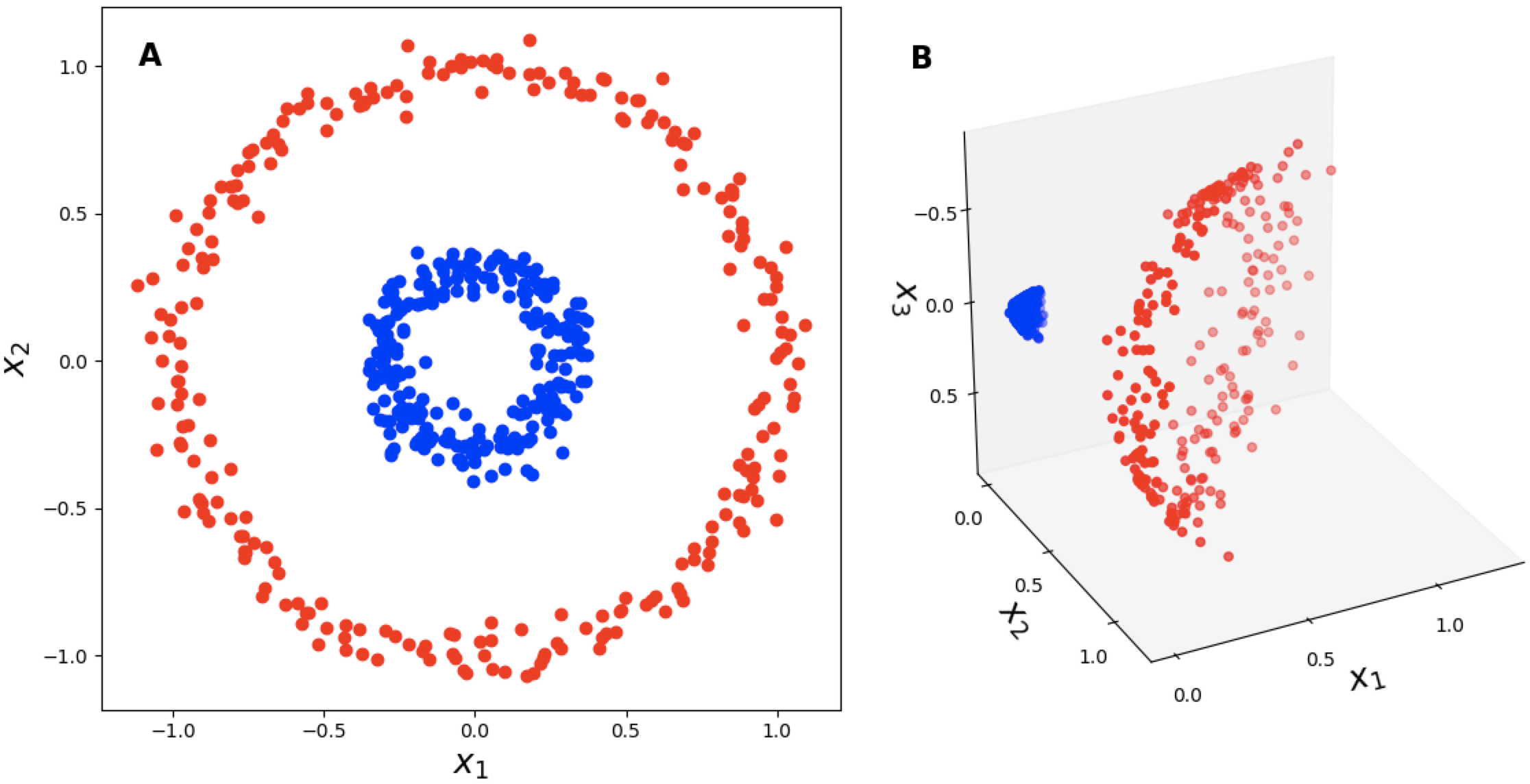
\(\rightarrow\) networks to add dimensions

Learning rate scheduling

• Change LR through training
• Typically: Quick warm up to target, then decay to zero
• Improved convergence

Python

schedule = keras.optimizers.schedules.CosineDecay(
  initial_learning_rate=1e-3
)
optimizer = keras.optimizers.Adam(learning_rate=schedule)

Issues with gradients

Gradients can become excessively large or vanishingly small

Exploding gradients

• Unstable training (jumping erratically)
• Numerical issues (overflow)

Remedies

• Batch normalization
• Gradient clipping

Vanishing gradients

• Slow training (barely moving)
• Numerical issues (underflow)

Remedies

• Batch normalization
• Different activation functions
• Residual connections

Batch normalization

• Keep output close to mean 0 and variance 1

Python

network = keras.models.Sequential([
    keras.Input((3,)),
    keras.layers.Dense(4, activation="relu"),
    keras.layers.BatchNormalization(),
    keras.layers.Dense(4),
    keras.layers.BatchNormalization(),
    keras.layers.Activation("relu"),
    keras.layers.Dense(2, activation="softmax")
])

Batch normalization

• Keep output close to mean 0 and variance 1

Python

network = keras.models.Sequential([
    keras.Input((3,)),
    keras.layers.Dense(4, activation="relu"),
    keras.layers.BatchNormalization(),
    keras.layers.Dense(4),
    keras.layers.BatchNormalization(),
    keras.layers.Activation("relu"),
    keras.layers.Dense(2, activation="softmax")
])

Gradient clipping

Scale down gradients if they exceed certain threshold

Value clipping

• Restrict gradients to a specified range
• Each gradient clipped individually

Norm clipping

• Restrict the size (norm) of the gradient to a specified range
• All gradients rescaled so that the norm becomes smaller

Python

optimizer=keras.optimizers.Adam(
  learning_rate=1e-3, 
  clipvalue=0.5,
  clipnorm=1.0)

Residual / skip connections

• Add output of a layer with its input
• Removes vanishing gradients
• Layer learns the “residual”: \(f(x) = r(x) + x\)

Python

inputs = keras.Input(shape=(64,))

residual = keras.layers.Dense(64)(inputs)
outputs = keras.layers.Add()([residual, inputs])
outputs = keras.layers.Activation("relu")(outputs)

outputs = keras.layers.Dense(10, activation="softmax")(outputs)

model = keras.Model(inputs, outputs)

Guards against overfiting

Large networks tend to overfit

Guards against overfiting

Large networks tend to overfit

Remedies

• Early stopping
• Regularization
• Dropout
• Add more data
• …

Early stopping

Early stopping

Python

early_stopping = keras.callbacks.EarlyStopping(
    monitor="val_loss",
    restore_best_weights=True 
)

model.fit(
    X_train, y_train,
    validation_data=(X_val, y_val),
    epochs=100,
    callbacks=[early_stopping]
)

Regularization

Add (weighted) norm of the parameters to the loss \[ \mathcal{L}(x, \theta) = \mathcal{L}_0(x, \theta) + \lambda ||\theta|| \]

L1

• \(||\theta||_1 = \sum|\theta|\)
• Encourages sparse weights
• Discourages large weights
• Feature selection/pruning

L2

• \(||\theta||_2 = \sum\theta^2\)
• Encourages spread out weights
• Discourages large weights

Regularization

Python

network = keras.Sequential([
    keras.layers.Dense(64, 
        activation="relu", 
        kernel_regularizer=keras.regularizers.l1(0.01)),
    keras.layers.Dense(32, 
        activation="relu", 
        kernel_regularizer=keras.regularizers.l2(0.02)),
    keras.layers.Dense(10, activation="softmax")
])

• In keras
  • kernel_regularizer: Weights
  • bias_regularizer: Bias
  • activity_regularizer: Layer output

Dropout

During training, “turn off” each activation with a probability \(p\)

Image source: learnopencv.com

• Better generalization
• Reduced dependence on single neurons
• Reduced expressiveness
• Increased variance during training

Dropout

Python

network = keras.Sequential([
    keras.Input((2,)),
    keras.layers.Dense(64, activation="relu"),
    keras.layers.Dropout(0.1),
    keras.layers.Dense(64, activation="relu"),
    keras.layers.Dropout(0.05),
    keras.layers.Dense(10, activation="softmax")
])

x = keras.random.normal((100, 2))

network(x)
network(x, training=True)

Dropout

Python

network = keras.Sequential([
    keras.Input((2,)),
    keras.layers.Dense(64, activation="relu"),
    keras.layers.Dropout(0.1),
    keras.layers.Dense(64, activation="relu"),
    keras.layers.Dropout(0.05),
    keras.layers.Dense(10, activation="softmax")
])

x = keras.random.normal((100, 2))

network(x)
network(x, training=True)

Special neural architectures

MLP

Pros

• Conceptually simple, universal function approximator
• Easy to train, established
• Almost zero assumptions about data

Cons

• Inefficient in high dimensions (many parameters)
• Works only with fixed size input/output
• Almost zero assumptions about data

Assumptions: Data types

Examples:

• Pictures
• Sequences (text, time-series)
• Sets

\(\rightarrow\) leverage properties of data to our advantage by building networks that make correct assumptions

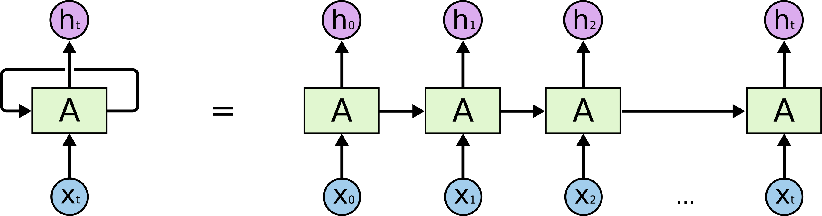
Recurrent neural network (RNN)

• Works for sequences of different lengths
• Maintain a hidden state \(h_t = \sigma_h(W_h * h_{t-1} + W_x x_t + b_h)\)
• Output depends on hidden state \(y_t = \sigma_y(W_g * h_t + b_y)\)

Issues

• Sequential updating
• Limited long-term memory
• Vanishing gradient

Source: Christopher Olah’s blog

Long short-term memory (LSTM)

• Learn to what to “forget” (forget gate) and what to “remember” (input gate)
• Cell state can carry over long term dependencies

Source: Christopher Olah’s blog

Attention (Vaswani et al., 2017)

• Sequential updating is slow
• Limited memory (even for LSTM)

Solution

• Use positional encoding (“concatenate with time variable”)
• Paralellize the whole computation
• “Attention”: Focus on the relevant parts of the sentence.

Attention

• Query: \(Q = XW_Q\)
• Key: \(K=XW_K\)
• Value: \(V=XW_V\)

\[ \text{Attention}(Q, K, V) = \text{softmax}(QK^{\text{T}})V \]

Attention

Attention

Attention

• Cross-attention
  • Keys and queries are computed from different sources
  • e.g., original (keys) and translated (queries) text
• Multihead attention
  • Multiple attention blocks in parallel
  • Each block “attends” to different representations
• Transformers: Multiple layers of Multihead attention layers and MLP

Set architectures

• What if we do not have a fixed order?
• Instead, we have sets

Set architectures

• Permutation invariant function: \(f(x) = f(\pi(x))\)

• Embeddings of sets

  • Handle different set sizes
  • Permutation invariant
  • Interactions between elements

Deep Set (Zaheer et al., 2017)

\[ f(X = \{ x_i \}) = \rho \left( \sigma(\tau(X)) \right) \]

• \(\tau\): Permutation equivariant function
• \(\sigma\): Permutation invariant pooling function (sum, mean)
• \(\rho\): Any function

Deep Set

Examples & further references

• Keras code examples
• Tensorflow playground
• Chollet (2021), GitHub
• Urban & Gates (2021)

References

Chollet, F. (2021). Deep learning with Python. Manning Publications.

Kingma, D. P., & Ba, J. (2014). Adam: A method for stochastic optimization. arXiv Preprint arXiv:1412.6980.

Kunc, V., & Kléma, J. (2024). Three decades of activations: A comprehensive survey of 400 activation functions for neural networks. arXiv Preprint arXiv:2402.09092.

Shahab, O., El Kurdi, B., Shaukat, A., Nadkarni, G., & Soroush, A. (2024). Large language models: A primer and gastroenterology applications. Therapeutic Advances in Gastroenterology, 17, 17562848241227031.

Urban, C. J., & Gates, K. M. (2021). Deep learning: A primer for psychologists. Psychological Methods, 26(6), 743.

Vaswani, A., Shazeer, N., Parmar, N., Uszkoreit, J., Jones, L., Gomez, A. N., Kaiser, Ł., & Polosukhin, I. (2017). Attention is all you need. Advances in Neural Information Processing Systems, 30.

Zaheer, M., Kottur, S., Ravanbakhsh, S., Poczos, B., Salakhutdinov, R. R., & Smola, A. J. (2017). Deep Sets. Advances in Neural Information Processing Systems, 30.