Amortized Bayesian Inference

with BayesFlow

Šimon Kucharský

Recap

Problem

We want to approximate \(p(\theta \mid x)\) or \(p(x \mid \theta)\)

\[ p(\theta \mid x) = \frac{p(\theta) \times p(x \mid \theta)}{p(x)} \]

• Evaluating \(p(\theta)\), \(p(x \mid \theta)\) and \(p(x)\) may not be tractable
• But we are able to sample \((x^{(s)}, \theta^{(s)}) \sim p(x, \theta)\)

Solution

Use generative neural networks

Inference network

• A generative neural network \(q_\phi(\theta \mid x)\)
  • Normalizing flow, flow matching, …
  • Model the distribution of parameters, conditioned on data

Goal:

\[p(\theta \mid x) \approx q_\phi(\theta \mid x)\]

Role of “data”

• \(x\) conditions the generative network
  • Normalizing flows: Input to coupling network (usually MLP)
  • Flow matching: Input to the vector field network (usually MLP)

\(\rightarrow\) Must be of fixed dimensions

Data of varying dimensions

• Sample sizes, study design, resolution, …

\(\rightarrow\) Summary statistics

1. Handcrafted: Mean, SD, Correlation,…
2. Summary networks

Summary network \(h_\psi\)

• Takes input of variable size
• Outputs fixed size embedding

\(\rightarrow\) Condition the inference network on the output of the summary network

\[p(\theta \mid x) \approx q_\phi(\theta \mid h_\psi(x))\]

Learning the posterior

\[ \begin{aligned} \hat{\phi}, \hat{\psi} = \operatorname*{argmin}_{\phi, \psi} & \mathbb{E}_{x \sim p(x)} \mathbb{KL}\big[p(\theta \mid x) || q_\phi(\theta \mid h_\psi(x))\big] = \\ = \operatorname*{argmin}_{\phi, \psi} & \mathbb{E}_{x \sim p(x)} \mathbb{E}_{\theta \sim p(\theta \mid x)} \log \frac{p(\theta \mid x)}{q_\phi(\theta \mid h_\psi(x))} \propto \\ \propto \operatorname*{argmin}_{\phi, \psi} & - \mathbb{E}_{(x, \theta) \sim p(x, \theta)} \log q_\phi(\theta \mid h_\psi(x)) \approx\\ \approx \operatorname*{argmin}_{\phi, \psi} & - \frac{1}{S}\sum_{s=1}^S \log q_\phi(\theta^{(s)} \mid h_\psi(x^{(s)})) \end{aligned} \]

\(\rightarrow\) must be able to generate samples \((x^{(s)}, \theta^{(s)}) \sim p(x, \theta)\)

Training the networks

1. Define a generative statistical model
   • \(p(x, \theta)\), typically \(p(\theta) \times p(x \mid \theta)\)
2. Define inference and (optional) summary networks
   • \(q_\phi(x \mid h_\psi(x))\)
3. Train the networks
   1. Sample from \((x^{(s)}, \theta^{(s)}) \sim p(x, \theta)\)
   2. Optimize weights \(\phi\) and \(\psi\) so that \(p(\theta \mid x) \approx q_\phi(\theta \mid h_\psi(x))\)

Inference

• Once the networks are trained, they can be used for inference
• Most of computational resources are used during training
• Inference is fast (only requires a simple pass through the network)

\(\rightarrow\) Amortized inference: Pay upfront the cost of inference during training, making subsequent inference effective

Amortized Bayesian Inference

For more info, see Radev et al. (2020)

Working with bayesflow

BayesFlow (Radev, Schmitt, Schumacher, et al., 2023)

• Python library
• Implementation of common neural architectures to make ABI easier
• Helper functions for simulation, configuration, training, validation, diagnostics,…

Old version

• Build on TensorFlow
• Previous projects build with it
• Bespoke syntax, not that transparent
• Stale development (no new features), being deprecated
• stable legacy branch on GitHub
• pip install git+https://github.com/bayesflow-org/bayesflow@stable-legacy

New version

• Built on keras
  • TensorFlow, JAX, or PyTorch as a backend
• Modern interface, more transparent, faster
• Released very recently
• Active development, future standard
• main branch on GitHub
• pip install git+https://github.com/bayesflow-org/bayesflow@main

General workflow

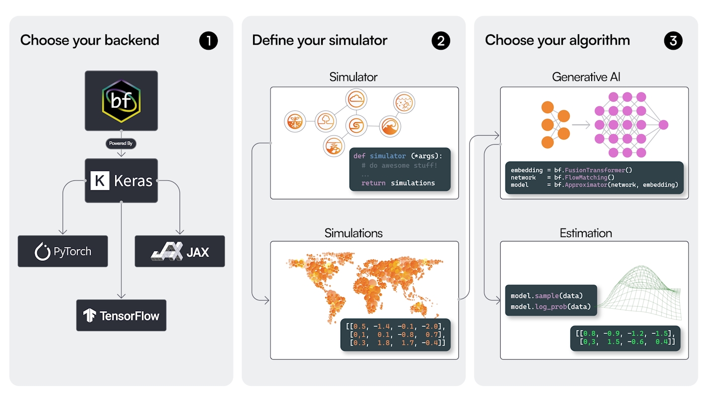
Ingredients

• Simulator
  • Simulate data from the statistical model
• Adapter
  • Configure the data
• Summary network (optional)
  • Get summary embeddings
• Inference network
  • Approximate the posterior

Quality of life

• Diagnostics
  • Plots and statistics to evaluate the approximation
• Approximator
  • Hold ingredients necessary for approximation together
  • Adapter, Summary network, Inference network
• Workflow
  • Hold ingredients for the entire pipeline together
  • Simulator, Adapter, Summary network Inference network, Diagnostics

General pipeline

1. Define the statistical model (through simulator)
2. Define the approximator (through neural networks)
3. Train the neural networks
4. Validate the approximator
5. Inference and diagnostics

1. Define the statistical model

Define the simulator

• Define the “statistical” model in terms of a simulator
• bayesflow expects “batched” simulations

Python

class Simulator(bf.simulators.Simulator):
    def sample(self, batch_size):
        theta = np.random.beta(1, 1, size=batch_size)
        x = np.random.binomial(n=10, p=theta)
        return dict(theta=theta, x=x)

simulator = Simulator()
dataset = simulator.sample(100)

Define the simulator

• Define the “statistical” model in terms of a simulator
• bayesflow expects “batched” simulations
• make_simulator: Convenient interface for “auto batching”

Python

def prior():
    return dict(mu = np.random.normal(0, 1))

def likelihood(mu):
    return dict(x = np.random.normal(mu, 1, size=20))

simulator = bf.make_simulator([prior, likelihood])

simulator.sample(10)

Simulator: Data of varying size

• The shape of data must be the same within each batch

Strategies:

1. Pad vectors to be the same length
2. Vary data shapes between batches

Pad/mask vectors

Python

def context():
    return dict(n = np.random.randint(10, 101))

def prior():
    return dict(mu = np.random.normal(0, 1))

def likelihood(mu, n):
    observed = np.zeros(0)
    observed[:n] = 1

    x = np.zeros(100)
    x[:n] = np.random.normal(mu, 1, size=n)
    return dict(observed=observed, x=x)

simulator = bf.make_simulator([context, prior, likelihood])

simulator.sample(10)

Vary data shape between batches

Python

def context(batch_size):
    return dict(n = np.random.randint(10, 101))

def prior():
    return dict(mu = np.random.normal(0, 1))

def likelihood(mu, n):
    x = np.random.normal(mu, 1, size=n)
    return dict(x=x)

simulator = bf.make_simulator([prior, likelihood], meta_fn=context)

simulator.sample(10)

Padding vs batched context

• Both approaches work
• Batched context is a bit cleaner
  • Do not have to fiddle with masking
  • Limited useability (cannot effectivelly use in offline mode)
• Padding
  • More verbose
  • More general

2. Define the approximator

Approximator

1. Inference network
   • Generates distributions
2. (Optional) summary network
   • Generates summary embeddings
3. Adapter
   • Reshapes data to be passed into networks

Inference network

Python

inference_network = bf.networks.CouplingFlow()

Python

inference_network = bf.networks.FlowMatching()

Various options available, see the Two Moons Example.

What architecture to pick?

Coupling flow

• Slow training
• Less expressive
• Faster during inference

Flow matching

• Fast training
• More expressive
• Slow inference on CPU

What architecture to pick?

• Affine coupling for low-dimensional, uni-modal posteriors
• Spline coupling for harder posteriors, including multi-modal
• Flow matching for highly complex posteriors
  • or when inference speed is not of concern
  • or if GPUs available

Summary network

• Extract all relevant information from the variable-sized data
• Output fixed sized embeddings
• “Sufficient statistics”
• Rule of thumb: output size should be at least \(2\times\) the number of parameters

What architecture to pick?

Reflect symmetries in the data

Exchangeable data

• Deep Sets, Set Transformers,…

Python

summary_network = bf.networks.DeepSet()

Time series, Sequences, …

• RNNs, CNNs, Transformers, …

Python

summary_network = bf.networks.LSTNet()

Adapter: Main purpose

• Reshapes data to be passed into networks
• A hub that handles what is passed into what network

Main keywords:

• "inference_variables": What are the variables that the inference network should learn about?
  • \(q(\theta \mid x) \rightarrow\) parameters \(\theta\)
• "inference_conditions": What are the variables that the inference network should be directly conditioned on?
  • \(q(\theta \mid x) \rightarrow\) data \(x\)
• "summary_variables": What are the variables that are supposed to be passed into the summary network?
  • \(q(\theta \mid f(x)) \rightarrow\) data \(x\)

Adapter

Python

adapter = (bf.Adapter()
  .concatenate(["mu", "sigma"], into = "inference_variables")
  .rename(["n"], "inference_conditions")
  .concatenate(["x", "observed"], into = "summary_variables")
)

• Transform variables
  • .standardize
  • .sqrt, .log
  • .constrain
• Reshape variables
  • .as_set, .as_time_series
  • .broadcast
  • .one_hot
• … and many more operations

Approximator

• Holds ingredients used for inference

Python

approximator = bf.approximators.ContinuousApproximator(
    inference_network=inference_network,
    summary_network=summary_network
    adapter=adapter
)

Workflow (optional)

• Hold all ingredients used for training, inference, and diagnostics

Python

workflow = bf.BasicWorkflow(
    inference_network=inference_network,
    summary_network=summary_network
    adapter=adapter,
    simulator=simulator
)

3. Train the neural networks

Network training

• In principle, training as any other model in keras

  • approximator.fit

• Define optimizer (e.g., keras.optimizers.Adam)

  • (optional) define schedule, early stopping,…

• Define training budget and regime

  • Number of epochs
  • Batch size, Number of batches
  • Simulate data or supply simulator

• Compile and train the model until convergence

• BasicWorkflow makes fitting easier, comes with some predefined reasonable settings

  • e.g. workflow.fit_online

Training regimes

Online

• Generate data during training
• Slower to train
• Prevents overfitting

Offline

• Train on fixed data
• Faster to train
• Risk of overfitting

From disk

• Offline training
• Large data that does not fit into memory
• Read data on demand during training

4. Validate the approximator

Goals

1. Is the neural approximator doing a good job at approximating the true posterior?
   • “Computational faithfulness”
   • Assesses the quality of approximator
2. How much can we expect to learn given data?
   • Parameter recovery, posterior contraction, posterior z-score
   • Assesses how the statistical model interacts with data

For general discussion, see Schad et al. (2021).

Procedure

1. Draw fresh validation data from the simulator
2. Extract the parameter samples from the prior
3. Sample from the posterior

Python

dataset = simulator.sample(1_000)
prior = {k: v if k in param_keys for k, v in dataset.items()}
posterior = approximator.sample(500, conditions = dataset)

Simulation-based calibration (SBC, Talts et al., 2018)

• Testing computational faithfulness of a posterior approximator
• Posterior distribution averaged over prior predictive distribution is the same as the prior distribution

\[ p(\theta) = \int \int p(\theta \mid \tilde{y}) \underbrace{p(\tilde{y} \mid \tilde{\theta}) p(\tilde{\theta})}_{\text{Prior predictives}} d\tilde{\theta} d \tilde{y} \]

Simulation-based calibration

1. Draw \(N\) prior predictive datasets \((\theta_i^{\text{sim}}, y_i^{\text{sim}}) \sim p(\theta, y)\)
2. For each data set \(y_i\), draw \(M\) samples from the approximate posterior: \(\theta_{ij} \sim q(\theta \mid y_i^{\text{sim}})\)
3. Calculate rank statistic \(r_i = \sum_{j=1}^M \text{I}\big(\theta_{ij} < \theta_i^{\text{sim}}\big)\)

Simulation-based calibration

Simulate

\[ \begin{aligned} \theta^{\text{sim}} & \sim p(\theta) \\ y^{\text{sim}} &\sim p(y \mid \theta^{\text{sim}}) \end{aligned} \]

By symmetry

\[ \begin{aligned} (\theta^{\text{sim}}, y^{\text{sim}}) & \sim p(\theta, y) \\ \theta^{\text{sim}} &\sim p(\theta \mid y^{\text{sim}}) \end{aligned} \]

Compute

\[ \begin{aligned} \theta_1, \dots, \theta_M & \sim q(\theta \mid y^{\text{sim}}) \\ \end{aligned} \]

If \(q(\theta \mid y^{\text{sim}}) = p(\theta \mid y^{\text{sim}})\), then the rank statistic of \(\theta^{\text{sim}}\) is uniform.

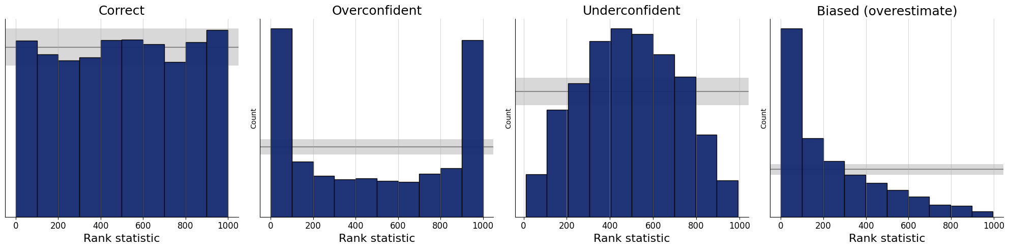
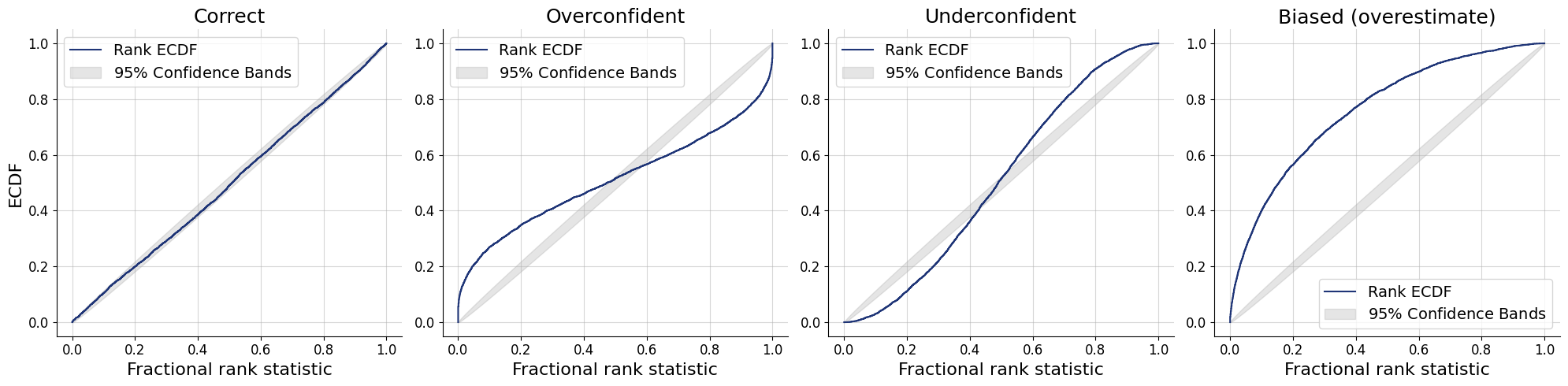
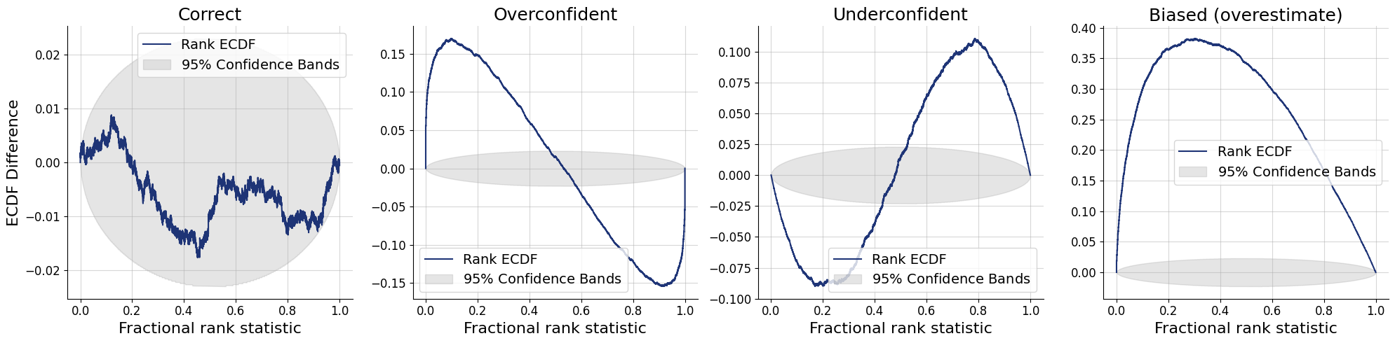
Visualizing SBC

1. Histograms
2. ECDF
3. ECDF difference

SBC Histograms

Python

fig=bf.diagnostics.calibration_histogram(
    estimates=posterior, 
    targets=prior)

SBC ECDF

Python

fig=bf.diagnostics.calibration_ecdf(
    estimates=posterior, 
    targets=prior)

SBC ECDF Difference

Python

fig=bf.diagnostics.calibration_ecdf(
    estimates=posterior, 
    targets=prior,
    difference=True)

SBC interpretation

• Necessary but not sufficient condition
  • ✅ All faithful approximators should pass the SBC check
  • ⚠️ An unfaithful approximator may pass the SBC check
• Depends on
  • Simulation budget (how many datasets)
  • Approximation precision (how many posterior draws per data set)
  • \(\rightarrow\) degree/ways of miscalibration, rather than ok/not ok

What if SBC check fails?

• Possible causes:
  • Underfitting \(\rightarrow\) increase expresiveness of inference or summary network, increase training budget
  • Overfitting \(\rightarrow\) decrease expressiveness of inference or summary network, increase training budget
  • Coding error \(\rightarrow\) check for errors in the simulator, setting up the approximator
  • Fundamental problem with the statistical model \(\rightarrow\) change the statistical model

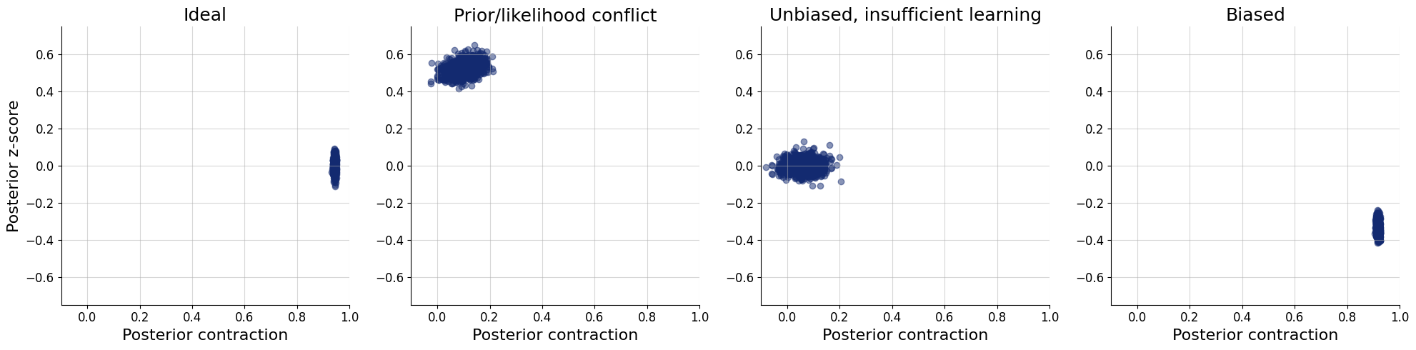
Posterior z-score

• How well does the estimated posterior mean match the true parameter used for simulating the data?

\[ z = \frac{\text{mean}(\theta_i) - \theta^{\text{sim}}}{\text{sd}(\theta_i)} \]

Posterior contraction

• How much uncertainty is removed after updating the prior to posterior?

\[ \text{contraction} = 1 - \frac{\text{sd}(\theta_i)}{\text{sd}(\theta^{\text{sim}})} \]

Z-score vs. contraction plot

Python

fig=bf.diagnostics.plots.z_score_contraction(
    estimates=posterior, 
    targets=prior)

Parameter recovery

• Plot the true parameter values \(\theta^{\text{sim}}\) against a posterior point estimate (mean, median)

Python

fig=bf.diagnostics.plots.recovery(estimates=posterior, targets=prior)

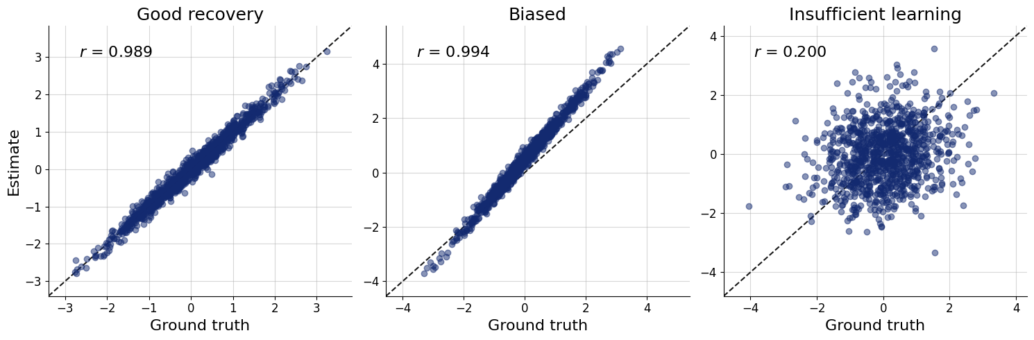
What if I get poor results

• Possible causes:
  • Poor calibration of the approximator \(\rightarrow\) see SBC
  • Poor identification of the parameters
    • Use more informative priors
    • Change the model
    • Add more data (sample size, additional variables)

5. Inference and diagnostics

Obtain posterior samples

Python

data = dict(y = ...)
posterior = approximator.sample(1000, conditions=data)

fig=bf.diagnostics.plots.pairs_posterior(estimates=posterior)

Model misspecification

• Prior misspecification
• Likelihood misspecification

\(\rightarrow\) Approximator may not be trusted

Posterior predictive checks

• Use posterior parameter posterior to simulate data from the simulator
• Compare simulated data to observed data
  • Visual checks - histograms, ecdf plots, scatter plots, …
  • Comparing summary statistics - means, variances, …

Use summary space

• Add a base distribution to the summary network, e.g.

Python

summary_network = bf.networks.Deepset(base_distribution="normal")

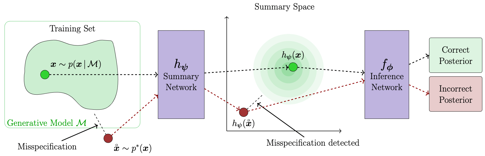
Schmitt et al. (2023)

Conclusion

Uses of BayesFlow

In addition to learning \(p(\theta \mid x)\):

• Generative modeling tasks
• Surrogate likelihood: \(p(x \mid \theta)\) (Radev, Schmitt, Pratz, et al., 2023)
• Model comparison: \(p(\mathcal{M} \mid x)\) (Elsemüller et al., 2024; Radev et al., 2021)
• Amortized point estimation: \(\hat{\theta}\) (Sainsbury-Dale et al., 2024)

Complex models

• Think about possible factorizations of the model
  • Split the problem into multiple smaller pieces
• Examples:
  • Multilevel models (Habermann et al., 2024)
  • Mixture models (Kucharský & Bürkner, 2025)

Advantages

• Fast inference
• Simulation based – intractable models

Disatvantages

• Need for training
• Simulation based – weaker guarantees

When to use ABI

• Fast inference needed, e.g.
  • Fitting hundreds of datasets
  • Online estimation (e.g., during an experimental setup)
• Intractable models

We do these things not because they are easy, but because we thought they were going to be easy.

— misquote of John F. Kennedy, unknown author

Resources:

• BayesFlow website: documentation, examples
• BayesFlow forum: ask questions about your use cases
• BayesFlow repository: contribute, submit bug reports, feature requests

References

Elsemüller, L., Schnuerch, M., Bürkner, P.-C., & Radev, S. T. (2024). A deep learning method for comparing bayesian hierarchical models. Psychological Methods, Advance online publication. https://doi.org/10.1037/met0000645

Habermann, D., Schmitt, M., Kühmichel, L., Bulling, A., Radev, S. T., & Bürkner, P.-C. (2024). Amortized bayesian multilevel models. arXiv Preprint arXiv:2408.13230.

Kucharský, Š., & Bürkner, P. C. (2025). Amortized bayesian mixture models. arXiv Preprint arXiv:2501.10229.

Radev, S. T., D’Alessandro, M., Mertens, U. K., Voss, A., Köthe, U., & Bürkner, P.-C. (2021). Amortized bayesian model comparison with evidential deep learning. IEEE Transactions on Neural Networks and Learning Systems, 34(8), 4903–4917.

Radev, S. T., Mertens, U. K., Voss, A., Ardizzone, L., & Köthe, U. (2020). BayesFlow: Learning complex stochastic models with invertible neural networks. IEEE Transactions on Neural Networks and Learning Systems, 33(4), 1452–1466.

Radev, S. T., Schmitt, M., Pratz, V., Picchini, U., Koethe, U., & Bürkner, P.-C. (2023). JANA: Jointly amortized neural approximation of complex bayesian models. The 39th Conference on Uncertainty in Artificial Intelligence. https://openreview.net/forum?id=dS3wVICQrU0

Radev, S. T., Schmitt, M., Schumacher, L., Elsemüller, L., Pratz, V., Schälte, Y., Köthe, U., & Bürkner, P.-C. (2023). BayesFlow: Amortized bayesian workflows with neural networks. arXiv. https://arxiv.org/abs/2306.16015

Sainsbury-Dale, M., Zammit-Mangion, A., & Huser, R. (2024). Likelihood-free parameter estimation with neural bayes estimators. The American Statistician, 78(1), 1–14.

Schad, D. J., Betancourt, M., & Vasishth, S. (2021). Toward a principled Bayesian workflow in cognitive science. Psychological Methods, 26(1), 103.

Schmitt, M., Bürkner, P.-C., Köthe, U., & Radev, S. T. (2023). Detecting model misspecification in amortized Bayesian inference with neural networks. DAGM German Conference on Pattern Recognition, 541–557.

Talts, S., Betancourt, M., Simpson, D., Vehtari, A., & Gelman, A. (2018). Validating bayesian inference algorithms with simulation-based calibration. arXiv Preprint arXiv:1804.06788.